Learning Objectives: The purpose of this set of exercises is to get acquainted with lighting and shading in WebGL and GLSL. We compute the local illumination of an object based on ambient, diffuse and specular material properties, and a light source.
When working on the following exercises, please consider the Wiki with clarifications for the textbook.
Tasks:
We can start this lab using the same code as presented in Part 2 of Worksheet 3, where three wireframe cubes are presented in perspective view. Let's get rid of the other cubes and switch to drawing triangles instead of wireframe by;
TRIANGLES in the render method
With this skeleton code we can now start implementing the exercise in the lab. This exercise is about using the technique known as recursive subdivision. This technique is used for approximations to curves and surfaces of a provided accuracy. This accuracy is determined by the amount of subdivisions (explained later). We with a tetrahedron composed of four equilateral triangles determined by the four vertices:
These vertices translated to code are:
var a = vec4(0.0, 0.0, 1.0, 1);
var b = vec4(0.0, 0.942809, -0.333333, 1);
var c = vec4(-0.816497, -0.471405, -0.333333, 1);
var d = vec4(0.816497, -0.471405, -0.333333, 1);
In order to make the tetrahedron we will be using the code that has been provided in the course book for the recursive subdivision. First thing that happens is that we take the origin points for the shape and send them to a function which will divide each of the faces into triangles as shown below:
function tetrahedron(a, b, c, d, n) {
        divideTriangle(a, b, c, n);
        divideTriangle(d, c, b, n);
        divideTriangle(a, d, b, n);
        divideTriangle(a, c, d, n);
    }
each of the phases can be divided into a number of triangles determined by the subdivision count. This subdivision count controls the exit condition to the following function which conducts the division of the triangle into sub triangles:
function divideTriangle(a, b, c, count) {
        if (count > 0) {
            var ab = normalize(mix(a, b, 0.5), true);
            var ac = normalize(mix(a, c, 0.5), true);
            var bc = normalize(mix(b, c, 0.5), true);

            divideTriangle(a, ab, ac, count - 1);
            divideTriangle(ab, b, bc, count - 1);
            divideTriangle(bc, c, ac, count - 1);
            divideTriangle(ab, bc, ac, count - 1);
        }
        else {
            triangle(a, b, c);
        }
    }
The final point to the recursive subdivision into triangles is the triangle function which will update the vertices that need to be rendered. This function is shown in the code below:
 function triangle(a, b, c) {
        vertices.push(a);
        vertices.push(b);
        vertices.push(c);

        index += 3;
    }
We can now render this tetrahedron directly on the screen using our skeleton code to have a shape as shown in the figure below (please note that each of the triangles are assigned a different color).
In order to add the two button to increase the number of subdivisions being made we have to reorganize our code so that the updated data can be rendered on screen. The buttons can be called using the following code:
// The button for increment the subdivision level
$("#btn-inc-1").click(function (e) {
    e.preventDefault();

    if (numSubdivisions == 6) {
        alert("Warning! \n Low performance from triangle count!")
    }

    numSubdivisions++;

    index = 0;
    vertices = [];
    normals = [];

    tetrahedron(a, b, c, d, numSubdivisions);

    updateUI();
    updateData();
    render();
});
// The decrement button
$("#btn-dec-1").click(function (e) {
        e.preventDefault();

        if (numSubdivisions <= 0) {
            alert("Subdivision count CANNOT be LOWER than 0!");
        } else {
            numSubdivisions--;

            index = 0;
            vertices = [];
            normals = [];

            tetrahedron(a, b, c, d, numSubdivisions);

            updateUI();
            updateData();
            render();
        }
})
The updateUI method simply writes to an HTML
p with the number of subdivisions being made. While the code
for the updateData is responsible for the
bufferSubdata calls being made to the shader. The
updateData is also responsible for assigning a new color to
the triangles being rendered using the following code:
        var triangle = -1;
        for (var i = 0; i < vertices.length; i++) {
            if (i % 3 == 0) {
                triangle++;

                if (triangle >= colors.length) {
                    triangle = 0;
                }
            }

            // Buffer the color data
            gl.bindBuffer(gl.ARRAY_BUFFER, colorBuffer);
            var color = vec4(colors[triangle]);
            gl.bufferSubData(gl.ARRAY_BUFFER, 16 * (i), flatten(color));
        }
0
Although it is a nice visual demonstration into seeing how the Recursive Subdivision works by having each of the individual triangles that are being drawn a different color, it is quite straining on the eyes to visualize the shape at high subdivision levels. Instead we can color the shape a rainbow of colors based on their position to see how face culling works.
To make this change will require the addition of the
gl_FragColor to be changed in the fragment shader to the
following formula:
gl_FragColor = 0.5 * fPosition + 0.5;
Doing so will require the addition of the fPosition varying
variable in both the fragment shader and the vertex shader. The position
should be passed after the position has been calculated by the following
code:
gl_Position = projectionMatrix * viewMatrix * modelMatrix * vPosition;
It also requires the enabling of face culling and depth check. Both of which are done simply by adding the following code:
gl.enable(gl.DEPTH_TEST);
gl.enable(gl.CULL_FACE);
gl.cullFace(gl.BACK)
gl.clear(gl.COLOR_BUFFER_BIT | gl.DEPTH_BUFFER_BIT);
The cullFace method is used to not draw parts of a 3D object
that are not visible to the camera, depending on what parameter we send.
In our case we see that sometimes when having large subdivision numbers we
get computer slowdown. Culling the back faces or the faces not towards the
camera can mitigate this a little bit as seen in the result below. For a
more in depth explanation on face culling see the
OpenGL
reference.
0
The result in Part 1 is flat shading in where all the triangles have a constant color assigned from the CPU. Where as the result from Part 2 all colors are rendered at the same lighting intensity making the viewer perceive the sphere as quite dull and unrealistic. As such we have to change the color values of the sphere depending on where the light source will be coming from. First we have to understand that lighting works by using a light source. These light-sources can be defined by the Illumination Function $I(x,y,z,\theta,\phi,\lambda)$ in where the variables are as follows:
This light-source will hit an object and alter the color that the human looking at it will perceive. In computer graphics we assume that most things can be colored with three different color components, $r,g,b$. Using these components we can obtain the corresponding color components that a human sees with the Luminance Function shown below:
$$ I=\begin{bmatrix} I_r \ I_g \ I_b \end{bmatrix} $$
When it comes to lighting an object it is not only the light that hits an object directly from a source but also the light that is reflected from scattered illumination around the room. It is unrealistic to try and calculate all objects reflecting light in a room. Instead computer graphics uses a principle that instead will have a baseline at which all objects in a room are light. This uniform lighting is called Ambient Lighting. This changes the luminance function to the following in where $I_a$ represents RGB light coming from the ambient.
$$ I=\begin{bmatrix} I_{ar} \ I_{ag} \ I_{ab} \end{bmatrix} $$
Lastly we can talk about how distant lighting works. Normally we would
have to calculate the $\theta,\phi$ vector for every point of an object to
understand how light is affecting the color of that object. However, with
distant lights we can instead assume that points that are close together
will be using a similar vector for the lighting. As such we do not have to
recalculate this vector. To let the computer know we assign
x,y,z
values to a light and follow it of with a 1 for close point light sources
or a 0 if it is a distant light.
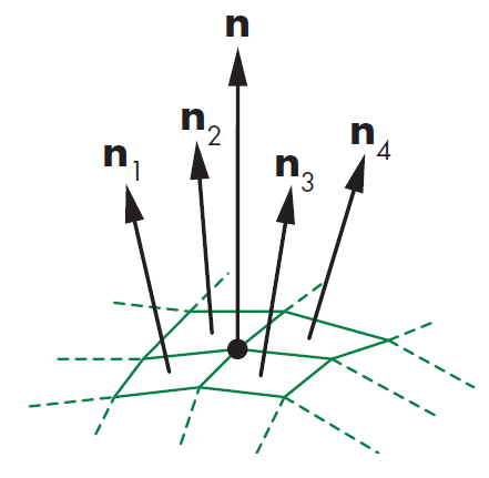
The lighting technique we will be using in this part of the lab is Gouraud Shading which can be used to achieve smooth lighting on low-polygon surfaces without having to calculate lighting for each pixel. This technique uses the calculation of surface normals which are perpendicular vertices to the object's surface. These normals are calculated at the vertex where polygons meet and the average normal is defined by the formula below:
$$ n = \frac{n_1 + n_2 + n3 + n_4}{|n_1 + n_2 + n3 + n_4|} $$
This means that each of the polygons that share that vertex will share the
normalized vector n which is the average of the polygon
normals as shown in the figure below:
Furthermore Gouraud's Model for shading says that with this average
normal at each vertex we can apply Phong Model to interpolate vertex
shades across each polygon. We will be by using an approximation of the
Phong Model as calculating the dot product of $$r \cdot v$$ for every
point will be computationally expensive. Instead calculating the
halfway vector between the viewer vector and the light-source
vector we can avoid the calculation of r by using the
following calculation:
$$ h=\frac{l+v}{|l+v|} $$
We can then avoid having to recalculate r for every point.
Instead use the halfway vector in the calculation for the spectacle term.
We have to additionally consider that the size of the specular highlights
will be smaller which can be mitigated by replacing the value of the
exponent e with a value e' so that $$(n
\cdot h)^{e`}$$ is closer to $$(r \cdot v )^e$$ making the intensities
similar.
In order to code this we need a way to keep track of what vertices make up a polygon. To do this we use a data structure that keeps track of polygons, vertices, normals , and material properties. We simply use variables in our JavaScript code and update them when creating each of the triangles to keep track of the true normals as seen below:
var pointsArray = [];
var normalsArray = [];

 // Create a single triangle
    function triangle(a, b, c) {
        var t1 = subtract(b, a);
        var t2 = subtract(c, a);

       // If using the calculated normals
       // var normal = normalize(cross(t2, t1));
       // normal = vec4(normal);

        // Else if using true analytical normals
        normalsArray.push(a);
        normalsArray.push(b);
        normalsArray.push(c);

        pointsArray.push(a);
        pointsArray.push(b);
        pointsArray.push(c);

        index += 3;
    }
We now have smooth shading in our result using these arithmetic calculated
normals. This solution will not be a full implementation of Gouraud
Shading though as the normals being sent are still the calculated normals
at each of the polygons. We instead need to calculate the average of these
normals at each vertex intercept. So to do this we can take the hint given
in the book and know that three polygons will intercept at the vertex
created for subdivision. Meaning that in the code above vertices
a,b,c correspond to three polygons each intercepting. The
simplest way to create a data structure that keeps track of the vertices
for each polygon is by implementing a 2D array where one dimension
represents each of the polygons and the other is each of the polygons'
vertices. Since we know that our polygons are triangles which are made at
this triangle method this is a trivial implementation if we use a object
orientated programming approach. First we make the class Polygon as shown
below:
var polygonArray = [];
class Polygon {
    constructor(va, vb, vc, name) {
        this.vertices = [va, vb, vc];
        this.name = name;
    }
}
Then we store the vertices of the polygon inside the
triangle method as shown below:
// Make each of the polygons using the vertex index number as identifier
var p = new Polygon(a, b, c, index);
polygonArray.push(p);
Now we can use the logging code below to make sure that each of the vertices only share three polygons which from the image below the code we see is true.
polygonArray.forEach(polygon => {
            polygon.vertices.forEach(vertex => {
                console.log("Vertex: "
                            + vertex
                            + " is the intersect between:");
                console.log("Polygon: " + polygon.name);
                polygonArray.forEach(polygon2 => {
                    if (polygon.name != polygon2.name) {
                        polygon2.vertices.forEach(vertex2 => {
                            if (vertex == vertex2) {
                                console.log("Polygon: " + polygon2.name);
                            }
                        });
                    }
                });
            });
        });
![[Pasted image 20221024113230.png]]
Making sure that our code is correctly identifying the polygons that share a vertex then we can apply the average function for normals and submit those to be used for Gouraud Shading as shown in the code below:
function findGouraudNormals() {
        var vertexNormals = [];
        polygonArray.forEach(polygon => {
            polygon.vertices.forEach(vertex => {
                vertexNormals.push(polygon.normal);
                polygonArray.forEach(polygon2 => {
                    if (polygon.name != polygon2.name) {
                        polygon2.vertices.forEach(vertex2 => {
                            if (vertex == vertex2) {
                                vertexNormals.push(polygon2.normal);
                            }
                        });
                    }
                });

                // // Calculate the average of the normals
                var sum;
                vertexNormals.forEach(n => {
                    if (sum == undefined) {
                        sum = n;
                    } else {
                        sum = add(sum, n);
                    }
                });

                var abs = vec4(Math.abs(sum[0]),
                            Math.abs(sum[1]),
                            Math.abs(sum[2]),
                            Math.abs(sum[3]));

                var normal = vec4(sum[0] / abs[0],
                                sum[1] / abs[1],
                                sum[2] / abs[2],
                                sum[3] / abs[3]);

                normalsArray.push(normal);

                // Reset the normals being looked at
                vertexNormals = [];
            });
        });
    }
We have now setup the calculation for the correct normals and can continue with the rest of the lab. As per the requirements of the lab we require to make our light source to be a white distance directional light. First we can start with declaring the distance and directional light. A light is directional instead of a point light if the last element in a vector is a 1 as stated previously, then the first three elements will determine the light's direction. So for a distant light in the direction $(0,0,-1)$ the code declaration will be:
var lightPosition = vec4(0.0, 0.0, -1.0, 0.0); // le
Now to determine the light color we use the light's ambient, specular, and diffuse properties. A white light is simply the presence of all RGB values so a white light with very little ambient light is declared as follows:
var lightAmbient = vec4(0.1,0.1,0.1,1.0); // la
var lightSpecular = vec4(1.0,1.0,1.0,1.0); // ls
var lightDiffuse = vec4(1.0, 1.0, 1.0, 1.0); // ld
Next in order to apply the Phong Model we need to declare the material properties which will make up the color that the object will take once light is reflected away. For our case the lab did not specify so we chose the following variables making the scene look like it's illuminating a planet we also change the clear color to black to fit this change:
var materialAmbient = vec4(1.0, 0.0, 1.0, 1.0); // k_a
var materialDiffuse = vec4(0.385, 0.520, 0.419, 1.0); // k_d
var materialSpecular = vec4(1.0, 1.0, 1.0, 1.0); // k_s
var materialShininess = 50.0;
gl.clearColor(0.1, 0.0, 0.1, 0.85);
We can now send the normalization and lighting variables to the vertex shader in the render method by using the following code:
 normalMatrix = [
    vec3(modelViewMatrix[0][0], modelViewMatrix[0][1], modelViewMatrix[0][2]),
    vec3(modelViewMatrix[1][0], modelViewMatrix[1][1], modelViewMatrix[1][2]),
    vec3(modelViewMatrix[2][0], modelViewMatrix[2][1], modelViewMatrix[2][2])
  ];

gl.uniformMatrix4fv(uniformLocations.normalMatrix, false, flatten(N));
gl.uniform4fv(uniformLocations.lightPosition, flatten(lightPosition));
With these variables being sent to the vertex shader we now have to implement these variables and use them to calculate the shading principles for the lighting. This is done by the following vertex shader code:
attribute vec4 vNormal; // Normals for each vertex
attribute vec4 vPosition; // Vertex positions

varying vec4 fColor;

// Lighting variables
uniform vec4 lightPosition;
uniform vec4 ambientProduct, diffuseProduct, specularProduct;
uniform float shininess;

// MVP matrices
uniform mat4 modelViewMatrix;
uniform mat4 projectionMatrix;

// Edge normals in accordance to eye coordinates
uniform mat3 normalMatrix;

void main() {
    // Convert the light and position of the vertex into eye coordinates
    vec3 pos = (modelViewMatrix * vPosition).xyz;
    vec3 light = lightPosition.xyz;

    // vector from vertex position to light source
    // Light determined if directional light or not
    vec3 L;
    if(lightPosition.w == 0.0) L = normalize(lightPosition.xyz);
    else L = normalize( lightPosition.xyz - pos );

    // Because the eye point is at the origin the vector from the vertex position to the eye is
    vec3 E = -normalize(pos);

    // halfway vector
    vec3 H = normalize( L + E );

    // Transform vertex normal into eye coordinates
    vec3 N = normalize( normalMatrix * vNormal.xyz );

    // Illumination equation
    vec4 ambient = ambientProduct;

    float KdLd = max( dot(L, N), 0.0);
    vec4 diffuse = KdLd * diffuseProduct;

    float KsLs = pow( max( dot(N,H), 0.0), shininess);
    vec4 specular = KsLs * specularProduct;

    if(dot(L,N) < 0.0) {
        specular = vec4(0.0,0.0,0.0,1.0);
    }

    gl_Position = projectionMatrix * modelViewMatrix * vPosition;

    // The part of code that gets sent to the fragment shader
    fColor = ambient + diffuse + specular;
    fColor.a = 1.0;
}
The effect is now shading the vertices of the shape using Gouraud Shading. The last request by the lab is to make the camera orbit around the object by simple adding the following code:
// Orbiting camera
var radius = 5;
var theta += 0.01;
var phi = 0.0;
eye = vec3(radius * Math.sin(theta) * Math.cos(phi)
           ,radius * Math.sin(theta) * Math.sin(phi)
           , radius * Math.cos(theta));
This code makes use of the eye part of the
viewMatrix in order to change the position of the camera. The
radius is the distance at which the camera will orbit around the object,
while theta is the change in angle every iteration. We can now call the
render method using the format we learned in Lab 1 of
window.requestAnimFrame(render) to continuously render the
changes.
0
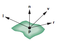
In the previous part we were using the modified Phong Reflection Model to get a quicker implementation of the Gouraud Model in this part we will use the full reflection model without calculating the half vectors in order to show what the Full Phong Reflection Model looks like. The Phong Model uses four vectors as shown in the figure below to calculate color for a point 'p' on the surface. The vector 'n' is the normal. The vector 'v' is in the direction from 'p' to the viewer. The vector 'l' is in the direction of the light source. The vector 'r' is the result of $$r = 2(l \times n)n - 1$$ which shows the angle of reflection.
When using the Phong Model we have to look at the following lighting conditions:
We have actually implemented most of this when implementing the Gouraud Model so now we have to get rid of the average vector calculation in the triangle method as shown below and go back to non interpolated normals:
var pointsArray = [];
var normalsArray = [];

 // Create a single triangle
    function triangle(a, b, c) {
        var t1 = subtract(b, a);
        var t2 = subtract(c, a);

       // If using the calculated normals
        var normal = normalize(cross(t2, t1));
        normal = vec4(normal);

        // Else if using true analytical normals
        normalsArray.push(a);
        normalsArray.push(b);
        normalsArray.push(c);

        pointsArray.push(a);
        pointsArray.push(b);
        pointsArray.push(c);

        index += 3;
    }
We can then add the sliders by following the HTML structure for a range input as shown below, where the label is used to tell the user what the current value of the variables are:
<div class="container-lbl">
    <label for="slide-kd-4">$$K_d$$</label>
    <p id="lbl-kd-4">= 0.5</p>
</div>
<input
id="slide-kd-4"
type="range"
min="0"
max="1.0"
step="0.1"
value="0.5" />
We can then implement them in JavaScript by using the
oninput method as shown below:
// The slider for the Le
    var sliderLe = document.getElementById("slide-Le-5");
    sliderLe.oninput = function () {
        $('#lbl-Le-5').text(" = " + this.value);
        le = this.value;
        index = 0;
        pointsArray = [];
        normalsArray = [];
        init();
    }
Which will update the variables used at the top of the
init function as shown below:
// The Slider variables
    var ka = 0.1;
    var kd = 0.4;
    var ks = 0.6;
    var al = 50.0;
    var le = 0.5;

lightAmbient = vec4(le / 10, le / 10, le / 10, 1.0);
lightDiffuse = vec4(le, le, le, 1.0);
lightSpecular = vec4(le, le, le, 1.0);

materialAmbient = vec4(ka, ka, ka, 1.0);
materialDiffuse = vec4(kd, kd, kd, 1.0);
materialSpecular = vec4(ks, ks, ks, 1.0);

materialShininess = al;
In order to have Phong shading we need to combine the Gouraud Shader and move the Phong Reflection Model calculations to be in the fragment shader so that instead of the vertices being assigned the color it is the polygon edges. This will flip our vertex and fragment shaders in the sense that the vertex shader will now be quite empty as normalizations will need to happen in the fragment shader. Below are the corresponding fragment and vertex shaders:
<script id="vertex-shader-5" type="x-shader/x-vertex">
attribute vec4 vPosition; // Vertex positions

// MVP matrices
uniform mat4 modelViewMatrix;
uniform mat4 projectionMatrix;

// Variables being sent to the fragment shader
varying mat4 fModel;
varying mat4 fProjection;
varying vec4 fNormal;
varying vec4 fPosition;

attribute vec4 vNormal; // Normals for each vertex

void main() {
    gl_Position = projectionMatrix * modelViewMatrix * vPosition;
    fNormal = vNormal;
    fPosition = vPosition;
    fProjection = projectionMatrix;
    fModel = modelViewMatrix;
}
</script>
<script id="fragment-shader-5" type="x-shader/x-fragment">
precision mediump float;

varying mat4 fModel;
varying mat4 fProjection;
varying vec4 fNormal;
varying vec4 fPosition;

// Lighting variables
uniform vec4 lightPosition;
uniform float shininess;

// Dot products of material and lighting variables
uniform vec4 ambientProduct;
uniform vec4 diffuseProduct;
uniform vec4 specularProduct;

// Edge normals in accordance to eye coordinates
uniform mat3 normalMatrix;

void main()
{
vec3 pos = (fModel * fPosition).xyz;

// check for directional light
vec3 L;
if(lightPosition.w == 0.0) L = normalize(lightPosition.xyz);
else L = normalize( lightPosition.xyz - pos );

vec3 E =  -normalize(pos);
vec3 N = normalize( normalMatrix*fNormal.xyz);


vec4 fColor;

vec3 H = normalize( L + E );
vec4 ambient = ambientProduct;

float Kd = max( dot(L, N), 0.0 );
vec4  diffuse = Kd*diffuseProduct;

float Ks = pow( max(dot(N, H), 0.0), shininess );
vec4  specular = Ks * specularProduct;

if( dot(L, N) < 0.0 ) specular = vec4(0.0, 0.0, 0.0, 1.0);

fColor = ambient + diffuse +specular;
fColor.a = 1.0;

gl_FragColor = fColor;
}
</script>
The Phong Reflection Model is a way of making an illumination of surfaces in order to simulate the way that surfaces reflect light. It breaks down reflection into three main aspects; ambient light, diffuse lighting, and specular reflection. It is calculated per vertex and gives a result which can be later interpreted by the fragment shader.
Phong Shading takes the result from the Phong Reflection model to produce a smooth shading technique to blend the colors of a shape at every pixel.
Flat shading is the simplest form of shading an object in where each of the polygons are given their own color by the application. Flat shading can give nice results and is simple to understand but requires a lot of manual labor by the programmer in order to get a nice result. Also flat shading results in just that shading that is less smooth at the edges of each polygon. Part 4 shows this type of shading.
Gouraud Shading takes the flat shading model and averages the shading of each neighboring polygon by taking the average of their normals then applies shading by using the modified Phong Model. This technique is fast to calculate by the computer and fast simple to implement by the programmer. However, it will be calculated in the application and therefore the CPU since it needs to keep track of the vertices in where polygons meet making it not desirable for real-time rendering of detailed scenes. Part 3 shows this type of shading.
Phong Shading builds upon Gouraud shading by finding the vertex normals and instead interpolates vertex average normals across edges and now interpolate the normals inside the polygon given the edge normals and apply the shading at every point corresponding to every fragment. Phong Shading will give a much smoother and accurate shading with less visible edges of the polygons. This type of shading is more work and also needs data structures to represent meshes to obtain the vertex normals. Part 5 shows this type of shading.
In order to simulate highlights the normalization of the vectors needs to be distinct enough that high values of the vector $l$ are allowed through. In special cases such as the apple shape there is a circular highlight that occurs known as a Specular Highlight which occurs because the colors around that spot are not being blended across it. This means that a shading system that depends on edge normals such as Gouraud Shading can sometimes blend across it and make this specular highlighting disappear. Making Phong Shading more desirable when it comes to highlights.
A point light is a light source with given positions in the scene it then illuminates the scene in every direction from it's surface. A point light's rays will fade out over a set distance. A light bulb is often used as analogous to a point light in the sense that a light bulb in your home will only illuminate objects around the light bulb not the entire home.
Directional light is supposed to represent a far away light ray originating at a light source. It is meant to be interpreted as coming from the same direction regardless of where the object or the viewer are. The most common analogy to a directional light is the sun. This is due to the sun being so far away we don't consider the location of the sun when calculating a shadow we instead understand the lighting from the sun as different rays that are hitting our planet. As such directional lighting is used for global lighting scenes in where every object is being affected in the same way by the directional light source.
Due to the eye position being key to the calculations such as the view direction, halfway vectors, and the normals. Changing the eye position will influence the illumination direction on the object making it be shaded in a different manner. This is most obvious with the specular highlights as moving the eye would make the highlight visible or invisible, as seen in the rotation of the sphere.
The Specular term of an object as described in the Phong Reflection Model is meant to refer the mirror properties of the object. A mirror is an object that reflects light in a narrow angle back to the viewer. If the specular term is set to 0 then the object will not reflect any light back resulting in no shine or highlights.
The shininess component is in control of the angle at which light is reflected the higher the value is the narrower the angle of reflection and thus the angle at which the reflection can be seen would be.
The book introduced the lighting in object space but later we see ways to make it more efficient by using local coordinate systems which is what were used for Part 3 through Part 5.
Lab Finished!
Report Finished!
Report Merged!